Simulating Bayes Factors: Extreme variability and absurd values?

Eric_Mah

I'm doing some Bayesian simulations (via R/BayesFactor) to better understand some data that I have, and have run into some strange results. Generated data is for a 2-group, between-subjects design (N = 500 per group, 10,000 samples generated) with a medium effect. Here's the code I used:

library(truncnorm)

seed <- round(runif(10000)*1000000)

makedata = function(x) {
  set.seed(x)
  #Generate condition 1 values
  a1 = rtruncnorm(500, a=0, b=1, mean = 0.55, sd = .22)
  #Generate condition 2 values
  b1 = rtruncnorm(500, a=0, b=1, mean = 0.46, sd = .26)
  a2 = as.data.frame(a1)
  b2 = as.data.frame(b1)
  a3 = a2 
  b3 = b2
  dat = bind_cols(a3, b3)
}

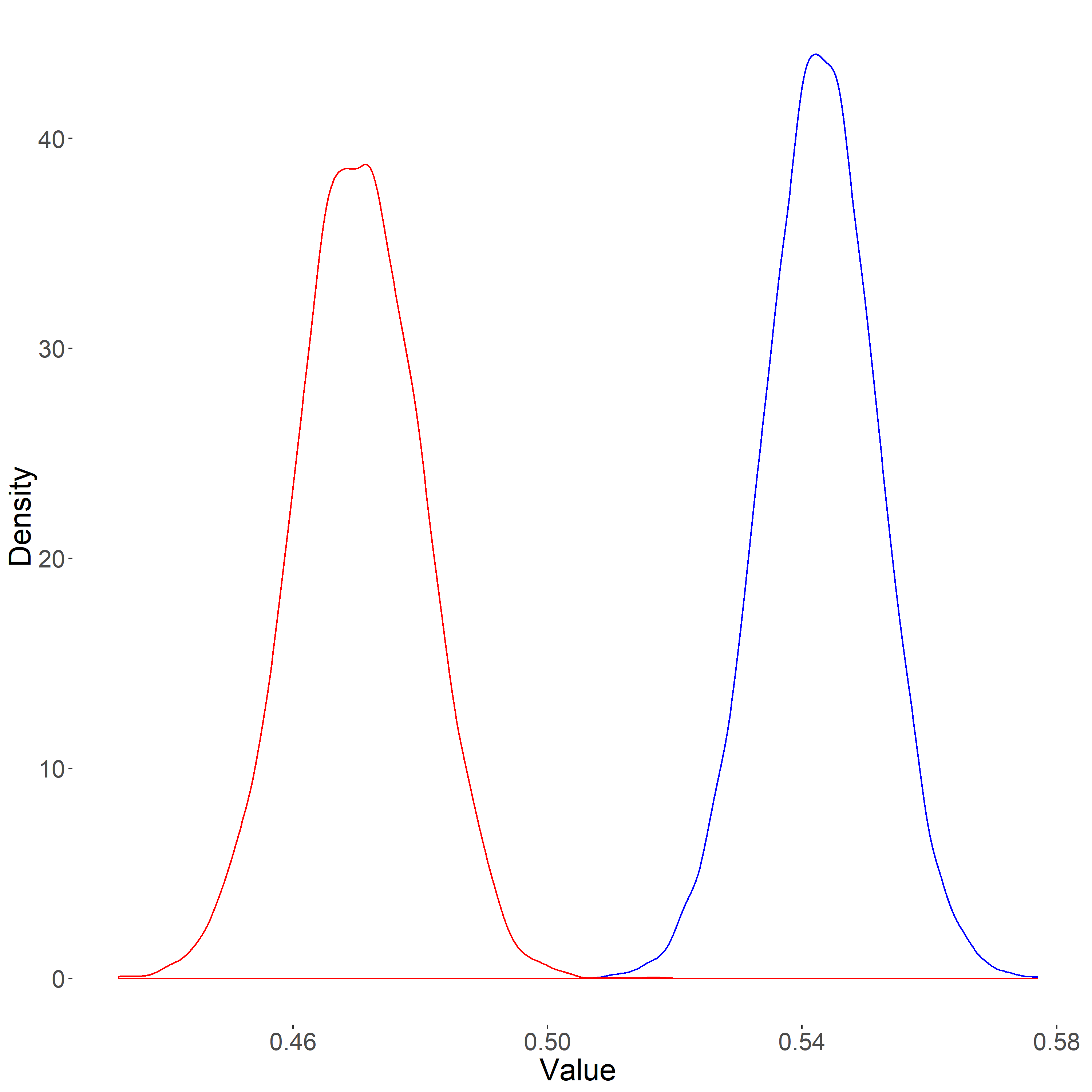
The distributions of condition means appear as expected:

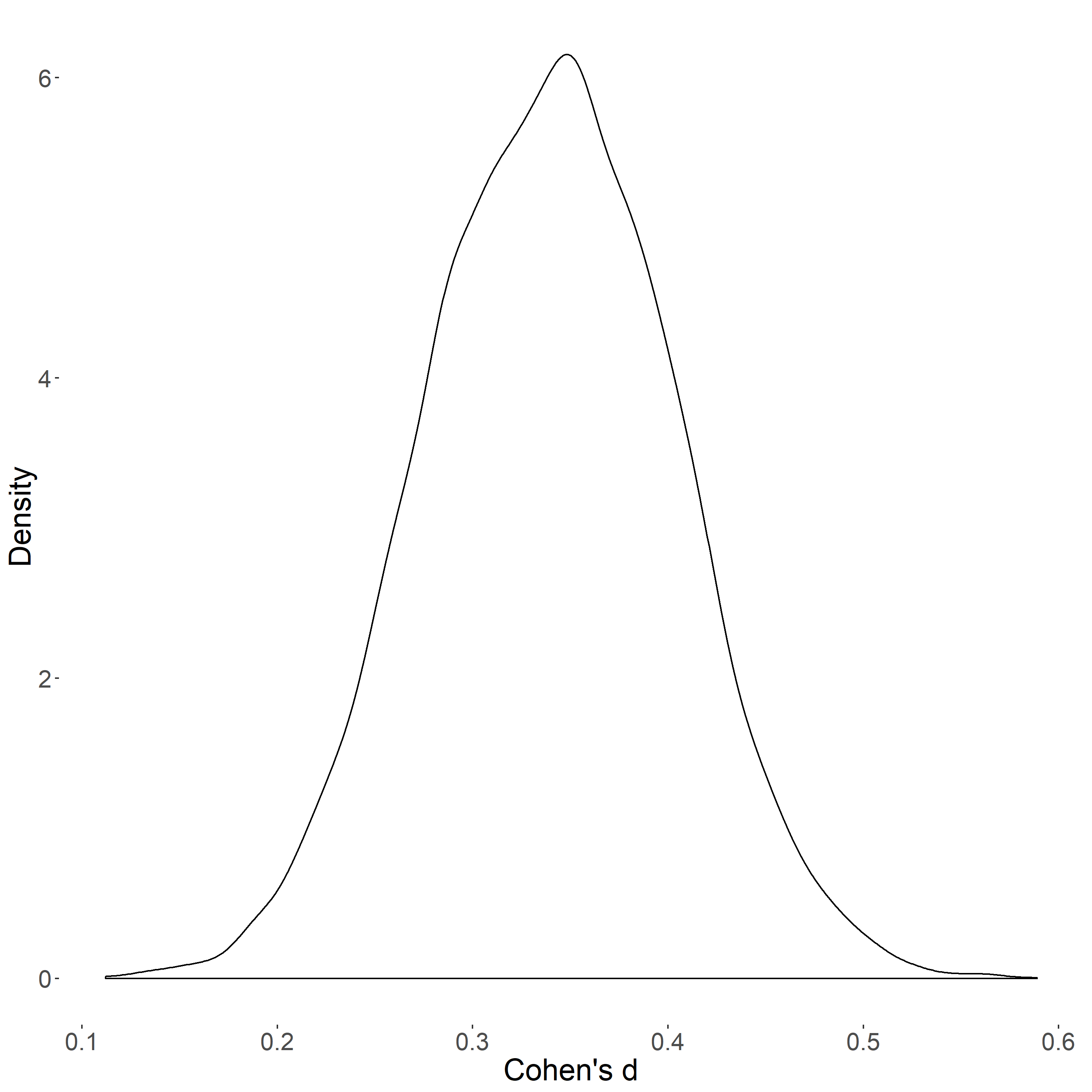
..and for the effect size distribution, the results are reasonable as well:

However, where it gets weird are the corresponding Bayes Factors for the mean differences. Here are the descriptives for the BF10s:

These values seem absurd (particularly the range/variability), at least given the seemingly reasonable values of group means and effect sizes. I'm aware that large BFs are possible with large samples/large effects, but I'm wondering if the higher variability in BFs is par for the course for Bayes Factors, or if something is going wrong with my simulations (which I'm happy to provide further details about). I've included the rest of the (highly unoptimized) code used to generate the datasets and means/effect sizes/BFs below:

datasets = lapply(seed, makedata) #Make datasets
BFresults = lapply(datasets, function(x) ttestBF(x = x$a1, y = x$b1, paired = FALSE)) #Bayesian t-tests for each dataset
BFresultsdata = lapply(BFresults, function(x) as.data.frame(x)) #Make them data frames
BFs = lapply(BFresultsdata, function (x) x[["bf"]]) #Get Bayes Factors
BFsD = as.data.frame(BFs)
BFsDT = as.data.frame(t(BFsD))
names(BFsDT) = c("BF10")
BFajrjcont1000 = BFsDT #Final data frame with all Bayes Factors

effresults = lapply(datasets, function(x) cohen.d(d = x$a1, f = x$b1, paired = FALSE)) #Effect sizes for each dataset
effsizes = lapply(effresults, function(x) x$estimate) #Get Cohen's ds
effsizesdata = as.data.frame(effsizes)
EffsDT = as.data.frame(t(effsizesdata))
names(EffsDT) = c("d")
Effajrjcont1000 = EffsDT #Final data frame with all Cohen's ds

ameanresults = lapply(datasets, function(x) mean(x$a1)) #Get condition 1 means
bmeanresults = lapply(datasets, function(x) mean (x$b1)) #Get condition 2 means
ameandata = as.data.frame(ameanresults) 
ameandataDT = as.data.frame(t(ameandata))
bmeandata = as.data.frame(bmeanresults)
bmeandataDT = as.data.frame(t(bmeandata))
meansdataajrjcont1000 = bind_cols(ameandataDT, bmeandataDT) #Final data frame with condition means

describe(BFajrjcont1000$BF10)
describe(Effajrjcont1000$d)
describe(meansdataajrjcont1000)

EJ

Hi Eric,

Two quick remarks:

1. Since BFs are defined as ratios, averaging them is problematic. For instance, assume data set 1 gives BF10 = 3, and data set 2 gives BF10 = 1/3. Overall, the data are nondiagnostic, but averaging 3 and 1/3 does not give 1. This is why people usually first apply a log transform before averaging.
2. When the effect size is large, and you have n=500, your BF can be huge. How huge depends on the height of the posterior distribution at delta=0. When the posterior distribution is peaked/far away from zero, this means that the effect depends on the tail of a distribution (which falls of exponentially). So yes, for whopper-sized effects, the absolute size of the BF can vary quite a bit. But I would argue that it does not matter that much whether BF = 10,000 or 1,000,000.

Cheers,

E.J.

Eric_Mah

E.J.,

Thanks for the reply! Looking at the descriptives and distribution of the log(BF10)s, things make more sense. To make sure I'm understanding the 2nd point correctly: is it that the variability in BF10s w/larger effects is due to the dependence on the tails of the posterior distributions, which are more sensitive to sample-to-sample changes than say, the peak?

Thanks!

Eric

EJ

Yes, that's right

Cheers,

E.J.