How to deal with the Infinite BF value?

Chen

I run a mixed-design Bayesian ANOVA in JASP. But I get an infinite inclusion BF value on one factor.

I have checked some posts on this issue. It seems that the models without this factor own a very very small posterior probability. But How can I solve this issue because I want to report the BF value in my article.

EJ

It would be useful to know what the numerical precision is for which the BF produces "infinity". There is an argument that the BF ought to be reported as "> x" where x is the maximum precision, instead of "infinity". Of course the inclusion probability is also not 1, it is 0.999999999 etc. Maybe a good topic for a feature request (https://jasp-stats.org/2018/03/29/request-feature-report-bug-jasp/). In the mean time, I would report it as "infinity" in the paper, and include a footnote saying that this represents a number so large that it exceeds the capacity of the computer. But I would nevertheless be interested in learning how large it is. I'll ask a team member.

EJ

vandenman

The maximum value of 64-bit float is 2^1024 * (1-2^(-53)) ~ 1.797693e+308. So I guess it would be fine to write BF > 2^2^10. However, the log Bayes factor tends to overflow to infinity more slowly, so perhaps it's better to report that one instead.

Chen

A great thank you to EJ and vandenman! 😘 Thank you for providing your suggestions!😊 They are really helpful!

I think currently I will consider to report an 'Inf' with some explanation on it. I do want to check if log(BF) will be a better choice. However, I re-run the analysis and I find, still, the value of inclusion BF on this factor is an Inf. Based on these results, I think maybe I can conclude that the effect of this factor is super necessary to explain the whole dataset because the models Without this specific factor are outperformed so badly.

Also, any supplement advice is welcomed!

Chen

I would like to add my finding for more related discussion. From the latest guideline book and also the previous post about the different approaches to acquire the BF, I get confused about which way is the best to calculate the BF, or, put it another way, how to compare models among the whole space when conducting the ANOVA in experiments with different extents of complexity.

From the article (Hinne et al., 2020, A Conceptual Introduction to Bayesian Model Averaging), it mainly suggest the model-averaging approach. But I still get very confused about how the JASP calculates the BF for interaction terms and main effect terms. Here, I want to first introduce what and why I am confused.

The Beginning

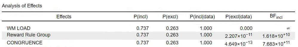
Lately I acquired an INF BF in my Bayesian ANOVA, as illustrated above. However, I notice that the BF I previously got, which was an INF, can be reduced to a value (still large though) after switching the setting of the comparison (an option of 'effect') from default "across all models" to "across matched models".

This actually has been specified in the previous studies, which implies that changing the approach to get the BF will influence the results of inclusion BFs. Moreover, it may increase and also may decrease the value of BFs.

Before that, I really want to verify what I've learned is correct. As I know, the approach of 'Across all models' averages all the models with and without the specific predictor and then calculates the BF. And the approach of 'across matched models', if I don't get it wrong, calculates interaction terms and main effect terms more targetedly.

As introduced in van den Bergh et al., 2018 (A Tutorial on Conducting and Interpreting a Bayesian ANOVA in JASP), for example, in a repeated ANOVA with two factors (A, B), to compute the BF for A × B interaction, the 'Across all models' uses the averaged inclusion probabilities of four models (including Null model, A model, B model, A+B model) to compare with the only model with interaction term (A + B + A×B model). However, 'Across matched models' compares only A + B model with A + B + A×B model to compute BF of the interaction term, and for main effect terms (not specified in the article), I think it compares only A with Null model to get the BF for main effect of A.

The question

Although it is rather easy to understand how it works for model-averaging approach and, if I get it right, the matched approach to calculate the interaction term, when the design increases the complexity (i.e., more factors), it is not so intuitive to know how the latter approach work in JASP. How does the matched approach work exactly?

And, as mentioned in Hinne et al. (2020), it seems to suggest using model averaging approach for many benefits. However, what if the complexity increases? If the model space extends to a large one, which approach is better? Back to the finding, if I use the matched approach, I can naturally constrain the comparison, which won't lead to a INF BF.

To lead to a broader question, in the context of conducting simple Bayesian ANOVA in the psychological studies, maybe it is not that important to consider the model uncertainty, which is one of the benefit of model averaging approach? Many of us are actually required to report the Bayesian statistics in our studies. Then what is the recommendation for computing the BFs?

EJ

Well, if you compare different models you get different BFs of course. What models you wish to compare is not a trivial matter. There is the issue of matched models, and there is the related issue of the principle of marginality (i.e., should it be the case that when a model features an interaction, it should also feature the constituent main effects?). I think that when you adhere to the principle of marginality, the matched models approach makes a little more sense to me.

Cheers,

E.J.