

Mousetrap Visualization Questions

I have a slew questions about visualization and mouse-tracking...
Given that these are mostly R questions and not OpenSesame questions, I realize that this might not be exactly the right place to ask it. That said, I did not know exactly where to ask this and I thought that a public forum would be better than a personal email in case anyone else has similar questions .
I suspect that some of my questions will be answered in the following paper (Kieslich et al., 2017. Mouse-and hand-tracking as a window to cognition: A tutorial on implementation, analysis, and visualization), though I don't think it's been published yet. I'm eagerly awaiting the paper.
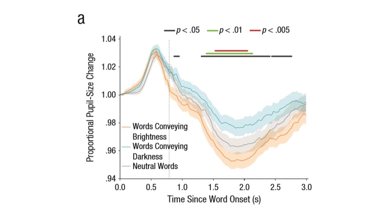
Question 1: Is there a way to add "confidence intervals" around the plots of MT trajectories? I'm thinking of a shaded band like in pupillometry studies (example is from Mathot, Grainger, Strijkers, 2017).
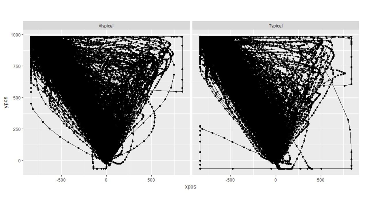
Question 2: How can we identify and remove individual trajectories? In the bottom right picture below, you can clearly see that there is a single trial than needs to be removed (the one that goes to the left and then all the way around hugging the edge). I know we can export a pdf of the individual trials and then eyeball them but is there a way to do this in R such that they can be "marked." Or do I simply have to match up the trajectory of the pdf with the row of the trial level data and then exclude that row?
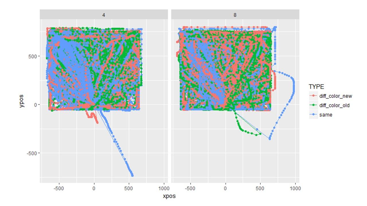
Question 3: I tried plotting the individual trajectories for a different experiment but something clearly went wrong. This makes me wonder if the plotted aggregate trajectories are off even though they look normal. I used the exact same sequence of code (shown below) for both the plots above and the plots below, yet it went haywire in this second one. I have no idea why. (Note the two experiments are completely different in design).
MT_DATA <- mt_import_mousetrap(d.CORR, timestamps_label= "timestamps_get_MT", xpos_label = "xpos_get_MT", ypos_label = "ypos_get_MT") MT_DATA <- mt_remap_symmetric(MT_DATA) MT_DATA <- mt_align_start(MT_DATA) MT_DATA <- mt_measures(MT_DATA) MT_DATA <- mt_time_normalize(MT_DATA, save_as="tn_trajectories", nsteps=101) MT_DATA <- mt_sample_entropy(MT_DATA, use="tn_trajectories", save_as="measures", dimension="xpos", m=3) plot_trials <- mt_plot(MT_DATA_FLINT, use="tn_trajectories", points = T, color = "TYPE", facet_col = "SIZE")
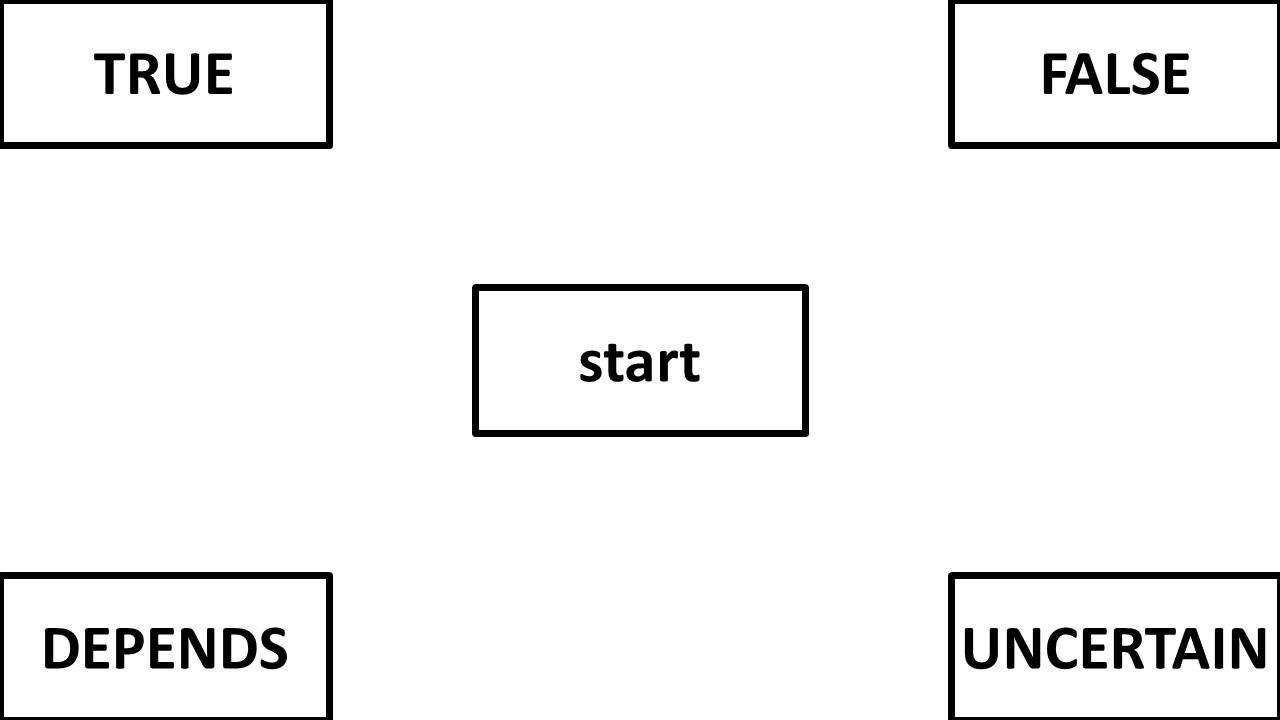
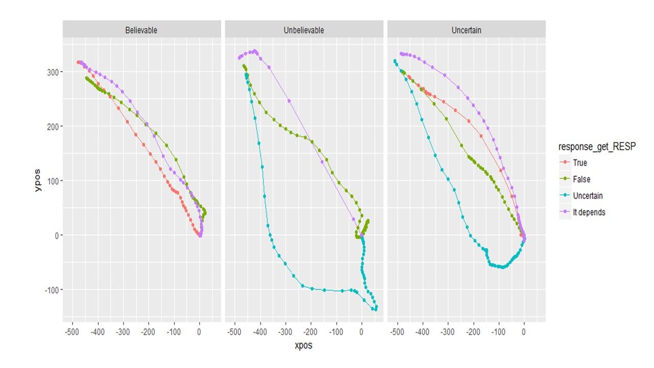
Question 4: What is the proper way to analyze/visualize a design with a 4 corner set up like the one below? My first thought in a design like this is to keep the responses in the same location rather than varying them across participants. My second thought is that I wouldn't necessarily want them to be symmetrically re-mapped either. Attraction towards false is (potentially) different than attraction towards uncertain. Then I wonder: will area under the curve or max deviation be accurately calculated if the trajectory initially goes up to "false" but then cuts diagonally and winds up going to "uncertain"? Would these changes be averaged out? Or should I consider a different DV like total_distance?
If I remap the data to be symmetric, it looks like this. (Note the data is only 60 trials of pilot data)
If I do NOT remap the data, it looks like this. And this seems more informative.
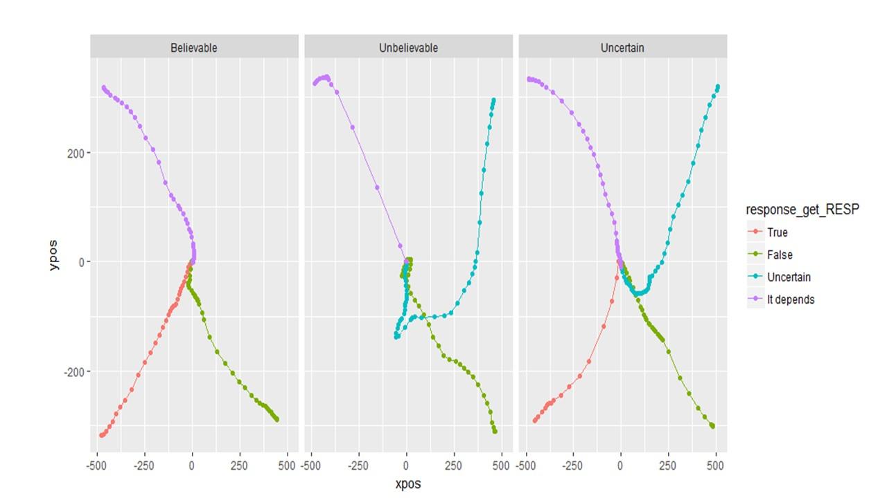
So if I choose to plot (and therefore analyze) unsymmetrical data, will the DVs (auc, MAD, etc) be calculated correctly?
Again, I apologize for the long post with numerous questions and I apologize if this thread is not in the correct location. Infinite thanks to any and all who can provide me with guidance on these questions!
Comments
Please note that in question 3 the last line of code mistakenly says MT_DATA_FLINT. That is a typo (and not the source of the error). It should be MT_DATA that gets passed into mt_plot. Apologies.
Hi Mike,
first off: sorry for the delayed reply - I was travling in the first half of November and lost a bit track of what was going on mousetrap-wise in the OpenSesame forum.
then: some meta-comments")
Good point about a place to ask mousetrap analysis related questions. I was thinking that it might make sense to have a separate forum for that (or maybe a subforum here - like there is one for PyGaze). I will think about it and also ask Sebastiaan what he thinks.
The mousetrap analysis paper you mentioned is still a working paper and unfortunately not quite finished yet. We will share a manuscript as soon as we have finished it - if you want to be notified once this happens you can sign up to our mousetrap mailing list: http://eepurl.com/co1AqX
I will answer your content questions in separate comments.
Best,
Pascal
Regarding question 1 (Is there a way to add "confidence intervals" around the plots of MT trajectories? )
yes, you can do this, e.g., of you plot the average x position of the time-normalized trajectory across time.
You can find a demonstration in the following example analysis that is documented online:
https://github.com/PascalKieslich/mousetrap-resources/blob/master/KieslichHenninger2017/KH2017_analyses_following_Dale_et_al.pdf
The relevant code is:
Aggregate time-normalized trajectories per condition separately per subject:
av_tn_trajectories <- mt_aggregate_per_subject(mt_data, use="tn_trajectories",use2_variables="Condition",subject_id="subject_nr")Plot aggregate trajectories with standard errors
(note that mean_se does not take into account within subjects design)
ggplot(av_tn_trajectories,aes(x=steps,y=xpos,group=Condition))+ stat_summary(geom = "ribbon",fun.data=mean_se,alpha=.2)+ geom_line(aes(color=Condition),stat="summary",fun.y="mean")+ scale_color_brewer(type="qual",palette = "Set1" )+ theme(legend.position=c(.2,.2))If you replace mean_se with mean_cl_normal or mean_cl_boot, you can get confidence bands. Note, however, that all of them are not exactly accurate as they assume a between subjects design. However, you could also calculate the CIs manually for the av_tn_trajectories data.frame.
Regarding question 2 (How can we identify and remove individual trajectories?):
There are different ways.
One way is to do as you suggested and to create a PDF of all individual trajectories using mt_plot_per_trajectory and inspect the trajectories. The plot provides the mt_id on each page which you could then use, e.g., in mt_subset to filter the trajectories.
An alternative way is to think about a mouse-tracking measure that might identify this trajectory. E.g., if you use mt_measures to compute the mouse-tracking measures for all trajectories, you could identify the trial as one of the only trials that has a xpos_max > 750. Specifically, you could use:
subset(mt_data$measures, xpos_max > 750)to check the mt_id of the trial.
Then you can plot it (assuming in the example below it has id12):
mt_plot(mt_data,subset=mt_id=="id12")If that is the trial, you can exclude it:
mt_data <- mt_subset(mt_data,mt_id!="id12")Note that you could also directly exclude all trials with xpos_max > 750 if you are sure that they should all be removed:
mt_data <- mt_subset(mt_data, xpos_max<=750, check="measures")Regarding question 3 (I tried plotting the individual trajectories for a different experiment but something clearly went wrong.)
Hmm, interesting. One idea I have is that the problem in the second case is that the coordinate system was not centered before you used mt_remap_symmetric. You might try whether it is enough for you to call mt_align_start before mt_remap_symmetric. If not, you would have to manually center the x and y positions. Happy to help in this case.
Regarding question 4 (What is the proper way to analyze/visualize a design with a 4 corner set up like the one below? ):
I actually spent quite some time exactly thinking about this") , i.e., the issue of calculating MAD/AUC/AD depending on whether the trajectories are remapped or not. I implemented it in mt_measures so that the values should be identical regardless of whether the trajectories are remapped or not. I also checked it for some example data. However, it would be great if you could also briefly look at this in your pilot data and let me know if they are identical for you as well.
, i.e., the issue of calculating MAD/AUC/AD depending on whether the trajectories are remapped or not. I implemented it in mt_measures so that the values should be identical regardless of whether the trajectories are remapped or not. I also checked it for some example data. However, it would be great if you could also briefly look at this in your pilot data and let me know if they are identical for you as well.
Hi Pascal,
First off, thank you for taking the time to answer my (numerous!) questions. I really appreciate it! I suspect your mousetrap work will explode in popularity and will soon need its own forum for questions. Also, thank you for connecting me with the mailing list.
Question1: The code you provided for the "confidence intervals" question was quite useful. I'm also glad to know that the bands are only for between subject designs. My current experiments are all fully within so I would have erred in my plots. Thanks for the save.
Question 2: Using the MT id method is a very efficient way to do things. I will definitely use this.
Question 3: I tried aligning the data before remapping it but it did not fix the problem. I still get the same strange plot. What's curious is that when I plot the aggregated data, it looks normal. (See below). Is it reasonable to assume that the aggregated plots can be trusted even though the individual trajectories aren't plotting properly? If so, then I'm not really sure how much time to spend figuring out this problem given that our hypothesized differences in trajectory didn't turn out and that this problem only occurs with this data set.
Question 4: I just checked my data and it turns out, the DVs are in fact identical regardless of whether the trajectories are remapped or not. I should have noticed this on my own. Nonetheless, this is good news and makes my life easier") . Now I know that remapping the data to make it symmetrical will affect how its plotted (and presented to the reader) but doesn't affect the calculation of the DVs for analyses. This is very good to know!
. Now I know that remapping the data to make it symmetrical will affect how its plotted (and presented to the reader) but doesn't affect the calculation of the DVs for analyses. This is very good to know!
I'm hoping that while we are having this conversation I can push my luck and ask one more question.
I've been uncertain about whether or not I've been processing time-sensitive measures (like velocity) appropriately.
Previously when I aggregated my data, I could not get some of the time DVs to work (e.g, vel_max or MAD_time). I would get an error saying that columns could not be found. Eventually, through much trial and error, I got it to work if I ran mt_derivatives, mt_deviations, and mt_average before running mt_measures. When I run mt_derivatives, mt_deviations **after **mt_measures, it does not work.
So now my normal order of operations is:
I just wanted to make sure that this order of operations is correct.
Finally, when I go to plot the velocities, I use the following code:
And I get a plot that looks like this;
So I try to aggregate it using the following code:
But I get the warning message:
I don't quite understand what this warning means or how grave it is. The plot it produces appears ok...
Also, is velocity measured in pixels? My plot above maxes out at 3 which seems low if this is measured in pixels.
Again, I appreciate your assistance and apologize for bombarding you with questions. I look forward to your forthcoming papers as I'm sure I'll have a better grasp of things afterwards.
Hi Mike,
glad to hear that most of the questions were solved!
Regarding question 3: I would definitely try to ensure that the plots of individual trajectories are accurate even when the aggregate plots look fine to prevent that problems wit data preprocessing on the trial level are masked by the aggregation procedure. Without the data at hand, it is a bit challenging for me to figure out the problem. If you want to, you can send me the data and your code via email (or probably bettere share a dropbox link with me via email) so I can try to figure out what is going on.
Best,
Pascal
Regarding the order of functions:
The order of running
makes sense.
Basically, mt_measures will return additional measures like max velocity and acceleration if it finds vel and acc in the data. We also document that in the function, but it is currently in the details section so we maybe should put it in a different place in the documentation.
Similarly, mt_average will average all dimenions that are present in the data until then.
Regarding the plots of average velocity:
The warning ("Trajectories differ in the number of logs. Aggregate trajectory data may be incorrect.") occurs, because you are plotting the average trajectories that contain a different number of recorded positions depending on the total duration of the trial (e.g., judging based on your figure above not many trials seem to have data for timestamps afteer 1200 ms). It would would not occur for time-normalized trajectories which all contain the same number of positions (and setting x="steps"). However, I think that it is often desired for velocity profiles to base them on average time bins of the raw trajectories as you are interested in the development of velocity across absolute time (and not relative time as in time normalized trajectories). You just have to keep in mind that for later periods of the trial less trajectories contribute to the aggregate trajectory that you are seeing which decreases comparability. One alternative could be to focus only on the time period were most trajectories still contain data (by specifying a max_interval in mt_average).
The unit of velocities is the unit of the x and y positions and timestamps, which is pixel and ms if you have used the mousetrap plugin in OpenSesame before. So a value 3 means 3 px per millisecond.
Thank you Pascal! You have been extremely generous with your time and patience in answering questions I should have figured out on my own.
I look forward to reading your forthcoming mouse-tracking papers and to (hopefully) the development of a MT specific forum!
Hi Pascal, I have a quick, and rather naive question, also related to the moustrap R package, so I thought I might just continue this thread. mt_measures uses the raw coordinates to compute measures of spatial attraction, but I am a bit confused as to whether these measures should be calculated from the time-normalized trajectories and if that matters. From what I can understand, in the Dale (2007) study you replicate in the mousetrap paper, they also analayze time-normalized trajectories. Freeman & Ambady (2010) refer to the importance of time-normalizing trajectories, but it is not clear to me whether it is important only because of visualization purposes, or if that should also be used to calculate the measures of spatial attraction. Thanks in advance!
By default, mt_measures calculates the measures using the raw trajectories, e.g., in the following code:
mt_example <- mt_measures(mt_example)You can also compute the measures based on the time-normalized trajectories:
mt_example <- mt_measures(mt_example,use="tn_trajectories")In practice, this does not make a difference for almost all measures - we report the correlation between measures based on time-normalized vs. raw trajectories here, they are all >.97 in our replication of Dale et al. (and for most measures even >.99).
Time-normalization is important mostly for visualization purposes (as you write above) or if you want to perform within trial analyses and analyse e.g. the development of the x position across time.