Odd: Bayesian Repeated Measures seems biased against interactions and in favor of main effects

sebastiaan

Edit: I should clarify that the problem (or what I perceive to be as such) is only with the inclusion Bayes Factor that you get when tick the 'Effects' box. The standard model-comparison table is fine.

I've been playing a bit with Bayesian Repeated Measures, mostly based on this question by @v.b. I used to think that I understood it fairly well, at least conceptually. But I can't wrap my head around the results that I describe below.

Follow me. We'll go by illustration.

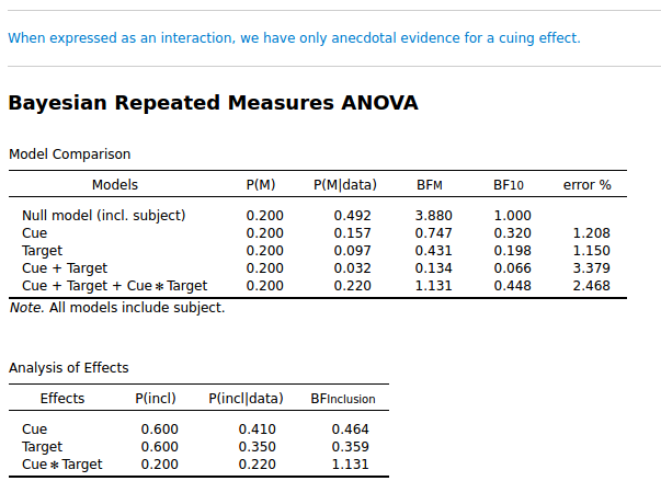
I simulated data from a Posner cuing experiment. (So this is fake data.) This is a 2 × 2 design: Cue (left/ right), and Target (left/ right). I simulated a small cuing effect, and as you can see below, it is not strongly supported: the inclusion BF for Cue × Target is 1.131. (I focus on the inclusion BF here, so the lower table.)

Ok. So far, nothing wrong.

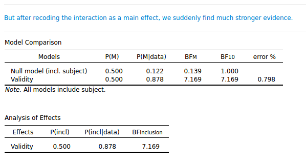
But it's a cuing effect, right? So another way to code the results is with a single factor: Validity (cue valid/ cue invalid). That shouldn't make any difference, right? And it doesn't make any difference in a traditional Repeated Measures, as you can see in the attached JASP file. But it makes a huge difference for the Bayesian analysis! If I collapse the valid and invalid columns from the data, and analyze it as a single-factor design, the inclusion BF for Validity is suddenly 7.169!

So a trivial recoding of the data brings us from anecdotal evidence to substantial evidence!

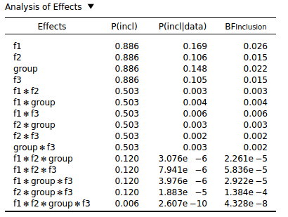
This seems to be a general property of Bayesian Repeated Measures: The more interactions an effect has, the lower the inclusion BF. You can see this with the following analysis that was conducted on purely random data:

I don't see how this behavior can be desirable. Surely all effects, regardless of whether they are interactions or main effects, should be given a fighting chance? But it seems that you are almost guaranteed to find evidence against interaction effects, especially higher-order interactions.

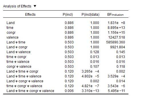
What is worse—but this I'm not sure about—I suspect that evidence in favor of main effects is exaggerated. I say this, because in the data of @v.b, the inclusion BFs for main effects are extremely high, while these same effects are not reliable in a traditional Repeated Measures:

I'm baffled.

On the one hand, the results of the Bayesian Repeated Measures seem invalid to me; on the other hand, I cannot believe that such an obvious problem would've gone undetected by anyone but me until now. So there are two options, both with a very low prior probability in my mind. Which makes me think that I fundamentally misunderstand what the output of the Bayesian Repeated Measures means.

Ideas, anyone?

EJ

A few quick responses:
1. Consider your very first example. The evidence for including the interaction (over the two main effects model) is .448/.066 = 6.79. I am not sure whether this will be exactly the same as the value from your recoded "validity" analysis (given that the BFs are estimated with uncertainty) but it's close.
2. The reason that the inclusion BF is around 1 is because the model with the interaction has to fight not just the two-main effects model, but also the null model and the models with only one main effect (and for this data set, these do pretty well).
3. By recoding to "validity" you have changed your model space. The single factor models "cue" and "target" no longer exist. Basically you have collapsed the model space and you are only assessing the interaction. Collapsing the model space will affect the inclusion BFs.
4. If you generate random data, you want the interactions to suffer more than the main effects, because the interaction models are more complex.
5. I will address the other issue in a moment. I think it might be due to the principle of marginality, which states that whenever an interaction is included, the constituent main effects need to be included as well.
E.J.

EJ

About the strong evidence for the main effects. A more informed assessment requires a look at the Bayes factors for the individual models. However, the Bayesian approach here is different from the classical approach, as it considers all of the possible models. What I see from the inclusion table is that the main effects are included in just about any model that gets support from the data. So the models without the variable "land" do very poorly. Note that, because of the principle of marginality, if a model excludes the main effect of "land", it also cannot have any interaction terms that involve "land".

I have seen this a few times before; an effect that is not reliable in the classical analysis gets strong support in a Bayesian setting. I suspect this occurs because the classical analysis does not compute all of the different models. Nevertheless, it would be great to figure it out. Maybe @v.b can send a recoded version of the data, or else PM us?

Cheers,
E.J.

sebastiaan

Let me start by stressing that this is the result that probability theory gives us.

(From this discussion.) Well, to paraphrase the creationists, probability theory is just a theory

No, but of course: I'm sure inclusion Bayes Factors have a valid interpretation in terms of probabilities. But this interpretation, or so it seems to me now, is very different from what most people would think.

What I get

As you say, if you just look at the model comparisons, then my simulated data has evidence for a cuing effect, regardless of whether it is coded as an interaction (BF = .448/.066 = 6.79; you get this by dividing the BF for the full model by that of the model without the interaction) or as a main effect (BF = 7.169). The numbers don't match exactly—but close enough.

It also makes perfect sense for me that—given purely random data—the BF against the null model decreases with increasing model complexity. This simply reflects that every addition to the model is a bad one, so the more we add, the further down the BF goes.

All that makes perfect sense to me.

What I don't get

But doing direct model comparisons works only because my example is a two-factorial design, in which case direct model comparisons are feasible. When you have four-factorial design, this is not feasible anymore.

And this is where I get confused: Because my understanding was that, for those multifactorial cases, inclusion BFs give conceptually the same information as you would get by doing direct model comparisons of the sort described above for the cuing effect. But they don't—clearly not. Rather, the inclusion BF for, say Cue x Target reflects (among other things) both the strength of the interaction and the strength of the main effects. This means that inclusion BFs are biased against crossover interactions, which don't have main effects. Right?

Or at least they are biased if you expect the inclusion BF for the interaction to reflect only the interaction.

Inclusion Baws Factor

I've been thinking a bit about what I would expect the inclusion BF to do. And here's what I came up with. To avoid confusion, let's call it the inclusion Baws Factor. Its official notation is

You determine the inclusion Baws Factor like this:

• If you want to know the evidence for an effect A
• You take all models that include A but no interactions with A
• For each model you divide the BF10 by the BF10 of the model that you get when you remove A
• Finally you take the average of all these division results.

That sounds kind of complicated, but it's not. To give an example, say that we have the following three-factorial analysis:

Edit: I forgot a few models here. See the continued discussion.

The inclusion Baws Factor for A×B would then be:

(BF[A+B+A×B] / BF[A+B]
+ BF[A+B+C+A×B] / BF[A+B+C])
/ 2
= .11

And for A it would be:

(BF[A]          / BF[null]
+ BF[A+B]       / BF[B]
+ BF[A+C]       / BF[C]
+ BF[A+B+C]     / BF[B+C]
+ BF[A+B+C+B×C] / BF[B+C+B×C])
/ 5
= .09

So the main effect of A and the two-way interaction A×B have more-or-less the same amount of evidence against them (.11 v .09). Which makes a lot of sense to me, because they are both equally non-existent.

This is not based on any deep insight! It's just what I, intuitively, would expect the inclusion Bayes Factor to do. Does that make sense?

EJ

OK I will address your comments one at a time. First off, yes, the inclusion BF need not give the same result as the direct model comparison. The direct comparison focuses on two models, and the inclusion BF averages across all of them.

You state: "This means that inclusion BFs are biased against crossover interactions, which don't have main effects. Right?" Again, the method is not biased; given the priors, the model, and the data, this is the unique end result. But let's consider the situation. You want an inclusion BF for an interaction. The prior probability for the interaction is not high, but what is relevant is the change from prior to posterior odds. The posterior probability for the interaction model benefits if the competition does not perform well. So with a cross-over interaction, the main effects will not receive much support, and therefore the inclusion BF should be higher for the cross-over interaction, not lower. I might be wrong of course -- human intuition is fallible. I'll respond to the Baws factor next.
E.J.

EJ

OK, I have briefly considered the Baws factor and I think it makes sense! However, I'd compute the result slightly differently. The problem is that you have to be careful about averaging BFs (e.g., the average of 1/3 and 3 is not 1). So suppose you want to determine the inclusion BF for a main effect A.
1. Take all models that include A but do not feature interactions with A.
2. Create a matching set of model by deleting A from each of the models defined in [1]
3. For this set of models, go through the regular inclusion BF procedure. This means that all models under consideration get equal prior probability, and that the BF10 for each model is computed and combined to yield posterior probabilities; you then compute the prior and posterior inclusion probabilities by summing across all "A" models and all "non-A" models. The change from prior to posterior odds is the inclusion BF.
Interesting.
E.J.

EJ

I just implemented the inclusion BF as one would for regression. For the case of ANOVA it is perhaps worthwhile to consider more carefully the kind of comparisons one would like to make. Different inclusion options could be made available in JASP. Would be worthwhile to ponder the interaction tests too.

sebastiaan

3. For this set of models, go through the regular inclusion BF procedure. This means that all models under consideration get equal prior probability, and that the BF10 for each model is computed and combined to yield posterior probabilities; you then compute the prior and posterior inclusion probabilities by summing across all "A" models and all "non-A" models. The change from prior to posterior odds is the inclusion BF.

It took me a while to figure out what you meant, but I think I got it. If I understand correctly, it's simply this:

 B) = sum(P[M|data] for each A-model) / sum(P[M|data] for each non-A-model)

Because there are just as many A-models als non-A-models, so we don't need to bother with P(M). Is my understanding correct?

I made a quick Python script to calculate from the model-comparison table, with Step 3 as I understand it now. This script is fully unchecked and based on a very limited understanding of Bayesian Statistics, so don't take it too seriously. (I'm not to be taken too seriously in general )

seems to behave sensibly, in the sense that it does not obviously favor or punish terms based on their complexity. The distribution of s is more-or-less the same for effects of different complexities when applied to random data, which I think makes sense.

When applied to @v.b 's data (sent by PM), the results are also more sensible (given my expectations) than for the inclusion BFs. However, there are still two terms that diverge uncomfortably from the traditional repeated measures: congruency × emotion and congruency × Land. (Rounding errors may also play a role here, because the model-comparison table has only 3-decimal precision.)

Edit: There was a bug in the previous table. Some models were taken into account which shouldn't have been. This is corrected now—I think. And it actually had surprisingly little effect on the results.

The SumPwith column is the sum of P[M|data] for all models with the relevant term; SumPwithout is the same for the models without. Nmodel indicates how many model-pairs are included in a given . So it's clearly not something you want to be doing by hand!

I just implemented the inclusion BF as one would for regression.

Is this too technical to explain here? If not, I'd be interested to know exactly how the inclusion BF differs for regression analyses.

sebastiaan

I quickly looked into the two Baws Factors that don't seem to match the p values. (In the process I also corrected a bug, so I updated the table above. The difference is small, though.)

For congruency×emotion, the Baws Factor is at least consistent with a direct model comparison:

BF10[congruency + emotion + congruency×emotion] = 5.119e90
/ BF10[congruency + emotion] = 4.595e91
= 0.11

This comes close to the Baws Factor of 0.09, even though it is based on (2×)50 models.

For congruency×Land, more-or-less the same story:

BF10[congruency + Land + congruency×Land] =  1.531e90
/ BF10[congruency + Land] = 3.331e86
= 4596

This also comes somewhat close to the Baws Factor of 12,492, even though (again) it is based on (2×)50 models.

So at least in these two cases, the Baws Factor gives results that match a more direct approach. For these effects, there seems to be a proper divergence between the Bayesian Repeated Measures and the traditional one; it's not just an artifact of

EJ

Hi Sebastiaan,
Yes, your understanding is correct. I think that the key aspect where your Baws Factor deviates from the inclusion BF is in the selection of the relevant models. For judging a main effect A, you disregard the models of higher complexity (i.e., those involving interactions with A). So I assume you propose something similar to assess interactions? So suppose I wish to test an AB interaction with the Baws Factor; the minimal model then also includes the individual main effects, so is [A + B + AB]. You then look at all models that include [A + B + AB] but do not include higher-order interactions involving [AB]. So you can have [A + B + C + AB]. And how about [A + B + C + AB + AC]? I think that should also be OK, right? But this one should not: [A + B + C+ AB + ABC], right?

In regression you just have K predictors that can each be in or out of the model. The inclusion BF takes a specific predictor and compares the summed posterior probability of all models that include that predictor against the summed posterior probability of all models that exclude it (there is a comparison to the prior odds in there as well, but this usually equals 1).

E.J.

sebastiaan

So I assume you propose something similar to assess interactions? So suppose I wish to test an AB interaction with the Baws Factor; the minimal model then also includes the individual main effects, so is [A + B + AB]. You then look at all models that include [A + B + AB] but do not include higher-order interactions involving [AB]. So you can have [A + B + C + AB]. And how about [A + B + C + AB + AC]? I think that should also be OK, right? But this one should not: [A + B + C+ AB + ABC], right?

Yes, that's correct. (My own example a few posts back was actually incomplete.) Below is what my script does. Say that we have an A×B×C design.

Models with:

• + contain the term of interest and are therefore included in the numerator
• - are what you get when you remove the term of interest from a + model and are therefore included in the denominator

And there's also a list of models that are excluded, because:

• They contain interactions with the term of interest; or
• Because they don't contain the term of interest, nor result from stripping the term of interest from a model that does contain the term of interest.

Main effect: A

Term: A

  Included models:
  + A
  - null

  + A + B
  - B

  + A + B + C
  - B + C

  + A + B + C + B*C
  - B + C + B*C

  + A + C
  - C

  Excluded models:
    A + B + A*B
    A + B + A*B + C
    A + B + A*B + C + A*C
    A + B + A*B + C + A*C + B*C
    A + B + A*B + C + A*C + B*C + A*B*C
    A + B + A*B + C + B*C
    A + B + C + A*C
    A + B + C + A*C + B*C
    A + C + A*C

Two-way interaction: A×B

Term: A*B

  Included models:
  + A + B + A*B
  - A + B

  + A + B + A*B + C
  - A + B + C

  + A + B + A*B + C + A*C
  - A + B + C + A*C

  + A + B + A*B + C + A*C + B*C
  - A + B + C + A*C + B*C

  + A + B + A*B + C + B*C
  - A + B + C + B*C

  Excluded models:
    A
    A + B + A*B + C + A*C + B*C + A*B*C
    A + C
    A + C + A*C
    B
    B + C
    B + C + B*C
    C
    null

Three-way interaction: A×B×C

Term: A*B*C

  Included models:
  + A + B + A*B + C + A*C + B*C + A*B*C
  - A + B + A*B + C + A*C + B*C

  Excluded models:
    A
    A + B
    A + B + A*B
    A + B + A*B + C
    A + B + A*B + C + A*C
    A + B + A*B + C + B*C
    A + B + C
    A + B + C + A*C
    A + B + C + A*C + B*C
    A + B + C + B*C
    A + C
    A + C + A*C
    B
    B + C
    B + C + B*C
    C
    null

sebastiaan

In regression you just have K predictors that can each be in or out of the model. The inclusion BF takes a specific predictor and compares the summed posterior probability of all models that include that predictor against the summed posterior probability of all models that exclude it (there is a comparison to the prior odds in there as well, but this usually equals 1).

It took me (as usual) a while to arrive at this insight, but: if I understand correctly, in the case of linear regression (or any set of models without interactions) the inclusion BF is the Baws Factor. It's just when interactions come in that the two start to diverge.

EJ

I think we might just add your ANOVA inclusion idea to JASP. Let me discuss this with the team. It is just another re-organization of the massive model table, with probability zero assigned to a specific subset of models.
E.J.

sebastiaan

That would be really cool! Let me know if I can help in some way.

Here's the Python script. I doubt it's very useful, if only because I wrote it as a chain of lambda expressions (brushing up on functional programming). But just in case.

• https://gist.github.com/smathot/68ecc023973b6a08e92163a80bc228f2